![[PyTorch tutorial] 파이토치로 딥러닝하기 : 60분만에 끝장내기](https://img1.daumcdn.net/thumb/R750x0/?scode=mtistory2&fname=https%3A%2F%2Fblog.kakaocdn.net%2Fdn%2FJAC3O%2FbtqD7Gvd0Da%2FmHTdnqhi7UZ3NTwbGK7CwK%2Fimg.png)
AUTOGRAD: 자동 미분
- 자코비안 행렬 소개 : 잘 정리된 영상이 있어서 킵
- 선형 변환 : x와 y축 각각 '한 칸'의 포인트가 선형으로 변환됨
- 좌표계의 변환, 해당 변환을 행렬로 표시할 수 있음
- 기저벡터 : [[1,0],[0,1]]
- 선형변환 : [[a,b],[c,d]]
- 넓이 : ad-bc (행렬식의 기하학적 의미)
- 비선형 변환 : radius / 세타 값으로 변환
신경망 정의하기
신경망 클래스 선언
import torch
import torch.nn as nn
import torch.nn.functional as F


class Net(nn.Module):

    def __init__(self):
        super(Net, self).__init__()
        # 1 input image channel, 6 output channels, 3x3 square convolution
        # kernel
        self.conv1 = nn.Conv2d(1, 6, 3)
        self.conv2 = nn.Conv2d(6, 16, 3)
        # an affine operation: y = Wx + b
        self.fc1 = nn.Linear(16 * 6 * 6, 120)  # 6*6 from image dimension
        self.fc2 = nn.Linear(120, 84)
        self.fc3 = nn.Linear(84, 10)

    def forward(self, x):
        # Max pooling over a (2, 2) window
        x = F.max_pool2d(F.relu(self.conv1(x)), (2, 2))
        # If the size is a square you can only specify a single number
        x = F.max_pool2d(F.relu(self.conv2(x)), 2)
        x = x.view(-1, self.num_flat_features(x))
        x = F.relu(self.fc1(x))
        x = F.relu(self.fc2(x))
        x = self.fc3(x)
        return x

    def num_flat_features(self, x):
        size = x.size()[1:]  # all dimensions except the batch dimension
        num_features = 1
        for s in size:
            num_features *= s
        return num_features


net = Net()
print(net)- forward 함수만 정의하고 나면, (변화도를 계산하는) backward 함수는 autograd 를 사용하여 자동으로 정의
- forward 함수에서는 어떠한 Tensor 연산을 사용해도 됨
- 모델의 학습 가능한 매개변수들은 net.parameters() 에 의해 반환
params = list(net.parameters())
print(len(params))
print(params[0].size())  # conv1's .weight
임의의 입력값
input = torch.randn(1, 1, 32, 32)
out = net(input)
print(out)
역전파
- 모든 매개변수의 변화도 버퍼(gradient buffer)를 0으로 설정하고, 무작위 값으로 역전파
net.zero_grad()
out.backward(torch.randn(1, 10))
Note
- torch.nn 은 미니-배치(mini-batch)만 지원합니다. torch.nn 패키지 전체는 하나의 샘플이 아닌, 샘플들의 미니-배치만을 입력으로 받습니다.
- 예를 들어, nnConv2D 는 nSamples x nChannels x Height x Width 의 4차원 Tensor를 입력으로 합니다.
- 만약 하나의 샘플만 있다면, input.unsqueeze(0) 을 사용해서 가짜 차원을 추가합니다.
요약
- torch.Tensor - backward() 같은 autograd 연산을 지원하는 다차원 배열 입니다. 또한 tensor에 대한 변화도(gradient)를 갖고 있습니다.
- nn.Module - 신경망 모듈. 매개변수를 캡슐화(encapsulation)하는 간편한 방법 으로, GPU로 이동, 내보내기(exporting), 불러오기(loading) 등의 작업을 위한 헬퍼(helper)를 제공합니다.
- nn.Parameter - Tensor의 한 종류로, Module 에 속성으로 할당될 때 자동으로 매개변수로 등록 됩니다.
- autograd.Function - autograd 연산의 전방향과 역방향 정의 를 구현합니다. 모든 Tensor 연산은 하나 이상의 Function 노드를 생성하며, 각 노드는 Tensor 를 생성하고 이력(history)을 부호화 하는 함수들과 연결하고 있습니다.
손실 함수(Loss Function)
- 손실 함수는 (output, target)을 한 쌍(pair)의 입력으로 받아, 출력(output)이 정답(target)으로부터 얼마나 멀리 떨어져있는지 추정하는 값을 계산
- nn 패키지에는 여러가지의 손실 함수들 이 존재함
- 예) nn.MSEloss : 출력과 대상간의 평균제곱오차(mean-squared error)를 계산
output = net(input)
target = torch.randn(10)  # a dummy target, for example
target = target.view(1, -1)  # make it the same shape as output
criterion = nn.MSELoss()

loss = criterion(output, target)
print(loss)- .grad_fn 속성을 사용하여 loss 를 역방향에서 따라가다보면, 이러한 모습의 연산 그래프를 볼 수 있음
input -> conv2d -> relu -> maxpool2d -> conv2d -> relu -> maxpool2d
-> view -> linear -> relu -> linear -> relu -> linear
-> MSELoss
-> loss
- loss.backward() 를 실행할 때, 전체 그래프는 손실(loss)에 대하여 미분되며, 그래프 내의 requires_grad=True 인 모든 Tensor는 변화도(gradient)가 누적된 .grad Tensor를 갖게 됨
역전파
- 오차(error)를 역전파하기 위해서는 loss.backward() 만 해주면 됨
- 이 때 기존 변화도를 없애는 작업이 필요한데, 그렇지 않으면 변화도가 기존의 것에 누적되기 때문
# 역전파 전과 후의 conv1의 bias gradient

net.zero_grad()     # zeroes the gradient buffers of all parameters

print('conv1.bias.grad before backward')
print(net.conv1.bias.grad)

#loss.backward() 호출
loss.backward()

print('conv1.bias.grad after backward')
print(net.conv1.bias.grad)
더보기
conv1.bias.grad before backward
tensor([0., 0., 0., 0., 0., 0.])
conv1.bias.grad after backward
tensor([ 0.0008, 0.0028, -0.0025, 0.0106, -0.0037, 0.0087])
가중치 갱신
- 확률적 경사 하강법(SGD; Stochastic Gradient Descent) : 가장 흔히 사용하는 갱신
learning_rate = 0.01
for f in net.parameters():
f.data.sub_(f.grad.data * learning_rate)- torch.optim 패키지 : SGD, Nesterov-SGD, Adam, RMSProp 등과 같은 다양한 갱신 규칙을 사용하고 싶을 때 사용
- SGD
- Adam
- Adadelta
- Adagrad
- AdamW
- SparseAdam
- Adamax
- ASGD (Averaged Stochastic Gradient Descent)
- RMSprop
- Rprop (resilient backpropagation)
import torch.optim as optim

# Optimizer를 생성합니다.
optimizer = optim.SGD(net.parameters(), lr=0.01)

# 학습 과정(training loop)에서는 다음과 같습니다:
optimizer.zero_grad()   # zero the gradient buffers
output = net(input)
loss = criterion(output, target)
loss.backward()
optimizer.step() # Does the update- optimizer.zero_grad() 를 사용하여 수동으로 변화도 버퍼를 0으로 설정하는 것에 유의
- 이는 역전파(Backprop) 섹션에서 설명한 것처럼 변화도가 누적되기 때문
이미지 분류기(Classifier) 학습하기
개요
PyTorch에서 이미지 데이터 활용을 위해서는 표준 python 패키지는 이용하여 Numpy 배열로 불러오면 됨
- 이미지는 Pillow나 OpenCV 같은 패키지가 유용
- 오디오를 처리할 때는 SciPy와 LibROSA가 유용
- 텍스트의 경우에는 그냥 Python이나 Cython을 사용해도 되고, NLTK나 SpaCy도 유용
- 특별히 영상 분야를 위해서는 torchvision이라는 패키지가 있음
- torchvision.datasets : 일반적으로 사용하는 데이터셋을 위한 데이터 로더(loader)
- torch.utils.data.DataLoader : 이미지용 데이터 변환기(transformer)
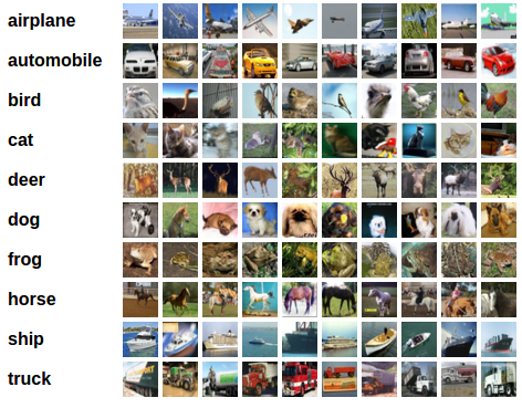
- CIFAR10 데이터셋 특성
- 카테고리 : ‘비행기(airplane)’, ‘자동차(automobile)’, ‘새(bird)’, ‘고양이(cat)’, ‘사슴(deer)’, ‘개(dog)’, ‘개구리(frog)’, ‘말(horse)’, ‘배(ship)’, ‘트럭(truck)’
- 이미지의 크기 : 3x32x32 (32x32 픽셀 크기의 이미지가 3개 채널(channel)의 색상로 이뤄져 있다는 뜻)
1. CIFAR10를 불러오고 정규화하기
import torch
import torchvision
import torchvision.transforms as transforms
transform = transforms.Compose(
[transforms.ToTensor(),
transforms.Normalize((0.5, 0.5, 0.5), (0.5, 0.5, 0.5))])
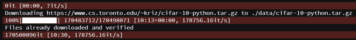
trainset = torchvision.datasets.CIFAR10(root='./data', train=True,
download=True, transform=transform)
trainloader = torch.utils.data.DataLoader(trainset, batch_size=4,
shuffle=True, num_workers=2)
testset = torchvision.datasets.CIFAR10(root='./data', train=False,
download=True, transform=transform)
testloader = torch.utils.data.DataLoader(testset, batch_size=4,
shuffle=False, num_workers=2)
classes = ('plane', 'car', 'bird', 'cat',
'deer', 'dog', 'frog', 'horse', 'ship', 'truck')- 아래와 같이 출력되며 data set이 다운로드됨
- 이미지 확인해보기
import matplotlib.pyplot as plt
import numpy as np

# 이미지를 보여주기 위한 함수

def imshow(img):
    img = img / 2 + 0.5     # unnormalize
    npimg = img.numpy()
    plt.imshow(np.transpose(npimg, (1, 2, 0)))
    plt.show()


# 학습용 이미지를 무작위로 가져오기
dataiter = iter(trainloader)
images, labels = dataiter.next()

# 이미지 보여주기
imshow(torchvision.utils.make_grid(images))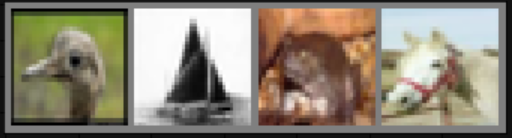
# 정답(label) 출력
print(' '.join('%5s' % classes[labels[j]] for j in range(4)))
# bird  ship  frog horse
2. 합성곱 신경망 적용하기
import torch.nn as nn
import torch.nn.functional as F


class Net(nn.Module):
    def __init__(self):
        super(Net, self).__init__()
        self.conv1 = nn.Conv2d(3, 6, 5)
        self.pool = nn.MaxPool2d(2, 2)
        self.conv2 = nn.Conv2d(6, 16, 5)
        self.fc1 = nn.Linear(16 * 5 * 5, 120)
        self.fc2 = nn.Linear(120, 84)
        self.fc3 = nn.Linear(84, 10)

    def forward(self, x):
        x = self.pool(F.relu(self.conv1(x)))
        x = self.pool(F.relu(self.conv2(x)))
        x = x.view(-1, 16 * 5 * 5)
        x = F.relu(self.fc1(x))
        x = F.relu(self.fc2(x))
        x = self.fc3(x)
        return x


net = Net()
3. 손실 함수와 Optimizer 정의하기
criterion = nn.CrossEntropyLoss()
optimizer = optim.SGD(net.parameters(), lr=0.001, momentum=0.9)
4. 신경망 학습하기
for epoch in range(2):   # 데이터셋을 수차례 반복합니다.

    running_loss = 0.0
    for i, data in enumerate(trainloader, 0):
        # [inputs, labels]의 목록인 data로부터 입력을 받은 후;
        inputs, labels = data

        # 변화도(Gradient) 매개변수를 0으로 만들고
        optimizer.zero_grad()

        # 순전파 + 역전파 + 최적화를 한 후
        outputs = net(inputs)
        loss = criterion(outputs, labels)
        loss.backward()
        optimizer.step()

        # 통계를 출력합니다.
        running_loss += loss.item()
        if i % 2000 == 1999:    # print every 2000 mini-batches
            print('[%d, %5d] loss: %.3f' %
                  (epoch + 1, i + 1, running_loss / 2000))
            running_loss = 0.0

print('Finished Training')- 꽤 오래 걸리는 편
- 모델 저장하기
#모델 저장하기
PATH = './cifar_net.pth'
torch.save(net.state_dict(), PATH)
5. 시험용 데이터로 신경망 검사하기
dataiter = iter(testloader)
images, labels = dataiter.next()

# 이미지를 출력합니다.
imshow(torchvision.utils.make_grid(images))
print('GroundTruth: ', ' '.join('%5s' % classes[labels[j]] for j in range(4)))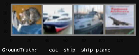
- 모델 불러오기
net = Net()
net.load_state_dict(torch.load(PATH)) #위에서 정의한 PATH- 신경망이 예측한 값 불러오기
- 예측모델의 출력은 10개 분류 각각에 대한 값으로 나타남
- 어떤 분류에 대해 더 높은 값이 나타난다는 것은 신경망이 그 이미지가 해당 분류에 더 가깝다고 생각하는 것
- 따라서, 가장 높은 값을 같는 인덱스를 뽑음
outputs = net(images)
_, predicted = torch.max(outputs, 1)

print('Predicted: ', ' '.join('%5s' % classes[predicted[j]]
                              for j in range(4)))]
#Predicted: cat car car plane- cat과 plane은 맞췄지만 ship은 둘 다 car로 예측
- 전체 데이터에 대한 정확도는?
#전체 데이터 셋을 적용한 정확도
correct = 0
total = 0
with torch.no_grad():
    for data in testloader:
        images, labels = data
        outputs = net(images)
        _, predicted = torch.max(outputs.data, 1)
        total += labels.size(0)
        correct += (predicted == labels).sum().item()

print('Accuracy of the network on the 10000 test images: %d %%' % (
100 * correct / total))- Accuracy of the network on the 10000 test images: 54 %
- 어떤 것을 잘 분류하고, 어떤 것을 더 못했는지
class_correct = list(0. for i in range(10))
class_total = list(0. for i in range(10))
with torch.no_grad():
    for data in testloader:
        images, labels = data
        outputs = net(images)
        _, predicted = torch.max(outputs, 1)
        c = (predicted == labels).squeeze()
        for i in range(4):
            label = labels[i]
            class_correct[label] += c[i].item()
            class_total[label] += 1


for i in range(10):
    print('Accuracy of %5s : %2d %%' % (
        classes[i], 100 * class_correct[i] / class_total[i]))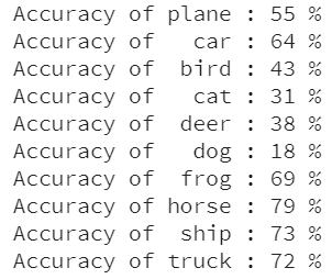
GPU에서 학습하기
device = torch.device("cuda:0" if torch.cuda.is_available() else "cpu")
print(device)
#cuda:0- 재귀적으로 모든 모듈의 매개변수와 버퍼를 CUDA tensor로 변경
net.to(device)- 각 단계에서 입력(input)과 정답(target)도 GPU로 보내야 함
inputs, labels = data[0].to(device), data[1].to(device)- Note : 신경망의 크기가 크지 않기 때문에 cpu에서 실행했을 때와 크게 차이가 나진 않음
'Undergraduate > ML & DL' 카테고리의 다른 글
| [Face Recognition] 얼굴 인식 출입, 어떻게 하는걸까? (0) | 2020.05.20 |
|---|---|
| [PyTorch tutorial] 컴퓨터 비전(Vision)을 위한 전이학습(Transfer Learning) (0) | 2020.05.14 |
| [GPU] 다수의 GPU 중 원하는 GPU 타겟팅하기 (0) | 2020.05.13 |
| [PyTorch tutorial] PyTorch에서 GPU 활용하기 (0) | 2020.05.12 |
| [PyTorch tutorial] 파이토치 설치하기 (0) | 2020.05.12 |